![]()
PEPit : numerical identification of worst-case examples
This notebook provides:
A simple example illustrating how to obtain a worst-case instance for gradient descent (when minimizing a smooth convex function) using the PEPit package.
Four other examples illustrating how to obtain worst-case instances in other situations: with proximal operators, momentum, possibly non-convex functions, and primal-dual methods.
For a first demo of PEPit, including detailed installation, imports, and basic introductory steps, we refer to the introductory demo file.
This notebook considers the following four algorithms:
Example 1 : gradient descent for smooth convex minimization (1D examples).
Example 2 : the fast iterative shrinkage-thresholding algorithm (FISTA) for composite convex minimization (1D examples).
Example 3 : gradient descent for smooth possibly non-convex minimization (1D examples).
Example 4 : an alternating projection algorithm for finding a point in intersection of two convex sets (2D examples).
Example 5 : a primal-dual proximal-point algorithm for convex (possibly non-smooth) minimization (2D examples).
Example 6 : gradient descent with exact line-search for smooth strongly convex minimization (2D examples).
Import a few necessary common Python packages (numpy, matplotlib)
import numpy as np
import matplotlib
matplotlib.rcParams.update({
    "mathtext.fontset": "cm",   # LaTeX font for rendering equations in plots
    "legend.fontsize": 12,
    "axes.labelsize": 14
})
import matplotlib.pyplot as plt

from math import sqrt
Table of Contents
We re-implement some basic examples below. This is necessary as we will save the worst-case trajectories.
Example 1 : gradient descent for smooth convex minimization
We consider the following convex minimization problem:
where \(f\) is \(L\)-smooth and convex.
For this example, we consider the problem of computing the smallest possible \(\tau(n, L, \gamma)\) such that the following guarantee holds (for any initialization of the algorithm, and any \(L\)-smooth convex functions)
where \(x_n\) is the output of gradient descent with fixed step size \(\gamma\), started from \(x_0\), and where \(x_\star\) is a minimizer of \(f\).
Algorithm
Gradient descent with fixed step size \(\gamma\) may be described as follows, for \(t \in \{0,1, \ldots, n-1\}\)
Low-dimensional worst-case examples
The solution to the PEP provides an example trajectory of points that would result in a worst-case convergence rate. In general, worst-case examples are non-unique in different ways: there are generally many trajectories of points that result in worst-case performance, and there are generally multiple different functions that can interpolate the same trajectory. Using a solution to the PEP, one can identify the dimension of a matching worst-case instance by inspection of the rank of the Gram matrix. More precisely, the rank of the Gram matrix corresponds to the dimension of the matching worst-case example (see, e.g., here, Section 3.2).
PEPit contains a few heuristics to try to identify such low-dimensional worst-case instances, by searching for low-rank Gram matrices. There are two of them: the trace heuristic (\(\ell_1\) on the eigenvalues) and the logdet heuristic—applying gradient descent on the logdet of the Gram matrix \(G\), which corresponds to a reweighted \(\ell_1\) on the eigenvalues of \(G\). For both of them, we need to potentially leave some slack in the objective, which we fix here to tol_dimension_reduction=1e-6.
from PEPit import PEP
from PEPit.functions import SmoothStronglyConvexFunction

L = 1
gamma = 1/L
n = 4
verbose = 1


# Instantiate PEP
problem = PEP()

# Declare a smooth strongly convex function
f = problem.declare_function(SmoothStronglyConvexFunction, L=L,mu=0)

# Then define the starting point x0 of the algorithm as well as corresponding gradient and function value g0 and f0
x0 = problem.set_initial_point()
g0, f0 = f.oracle(x0)

xs = f.stationary_point()
gs, fs = f.oracle(xs)

# Prepare empty lists for saving all datapoints
x_list = list()
g_list = list()
f_list = list()

# Run n steps of GD method with step-size gamma
gx, fx = g0, f0

x_list.append(x0)
g_list.append(g0)
f_list.append(f0)

for i in range(n):
    x_list.append(x_list[-1] - gamma * gx)
    gx, fx = f.oracle(x_list[-1])
    g_list.append(gx)
    f_list.append(fx)

# Set initial condition and performance metric
problem.set_initial_condition((x0-xs)**2 <= 1)
problem.set_performance_metric(f_list[-1] - fs)

# Solve the PEP
pepit_verbose = max(verbose, 0)
pepit_tau = problem.solve(verbose=pepit_verbose, dimension_reduction_heuristic="trace", tol_dimension_reduction=1e-6)
(PEPit) Setting up the problem: performance measure is the minimum of 1 element(s)
(PEPit) Setting up the problem: Adding initial conditions and general constraints ...
(PEPit) Setting up the problem: initial conditions and general constraints (1 constraint(s) added)
(PEPit) Setting up the problem: interpolation conditions for 1 function(s)
			Function 1 : Adding 30 scalar constraint(s) ...
			Function 1 : 30 scalar constraint(s) added
(PEPit) Setting up the problem: additional constraints for 0 function(s)
(PEPit) Setting up the problem: size of the Gram matrix: 7x7
(PEPit) Compiling SDP
(PEPit) Calling SDP solver
(PEPit) Solver status: optimal (wrapper:cvxpy, solver: MOSEK); optimal value: 0.05555555533811466
(PEPit) Postprocessing: 2 eigenvalue(s) > 4.671407470112186e-08 before dimension reduction
(PEPit) Calling SDP solver
(PEPit) Solver status: optimal (solver: MOSEK); objective value: 0.055554555299553596
(PEPit) Postprocessing: 1 eigenvalue(s) > 1.7470776746371454e-09 after dimension reduction
(PEPit) Postprocessing: solver's output is not entirely feasible (smallest eigenvalue of the Gram matrix is: -4.18e-11 < 0).
 Small deviation from 0 may simply be due to numerical error. Big ones should be deeply investigated.
 In any case, from now the provided values of parameters are based on the projection of the Gram matrix onto the cone of symmetric semi-definite matrix.
(PEPit) Primal feasibility check:
		The solver found a Gram matrix that is positive semi-definite up to an error of 4.1801938146378587e-11
		All the primal scalar constraints are verified up to an error of 7.835664582456214e-11
(PEPit) Dual feasibility check:
		The solver found a residual matrix that is positive semi-definite
		All the dual scalar values associated with inequality constraints are nonnegative up to an error of 2.8401468021662646e-09
(PEPit) The worst-case guarantee proof is perfectly reconstituted up to an error of 4.100136013346356e-08
(PEPit) Final upper bound (dual): 0.05555555838910858 and lower bound (primal example): 0.055554555299553596
(PEPit) Duality gap: absolute: 1.0030895549809071e-06 and relative: 1.805593707972616e-05
As we can see from the output, PEPit identified a low-rank matrix where all eigenvalues (except one) is approximately equal to 0. This corresponds to a single-dimensional worst-case example.
In order to evaluate and plot a worst-case trajectory, we use the eval function on the iterates, their gradients, and function values. Since we want to visualize the worst-case in 1D, we trim the dimension to only the first components.
# Evaluate the iterations:

x_list_evaluated = [x.eval()[0] for x in x_list] # [0] is because we are interested in largest component only
g_list_evaluated = [g.eval()[0] for g in g_list] # same
f_list_evaluated = [f.eval() for f in f_list]

# Evaluate specific points (for better visualization later)
xs_evaluated = xs.eval()[0] # x*
gs_evaluated = gs.eval()[0] # g(x*)=0
fs_evaluated = fs.eval() # f(x*)

x0_evaluated = x0.eval()[0] # x0
g0_evaluated = g0.eval()[0] # g(x0)
f0_evaluated = f0.eval() # f(x0)
Now, using the list of iterates, we can simply plot the trajectory (in terms of \((x,f(x))\) as follows:
plt.plot(x_list_evaluated, f_list_evaluated, '.--', color='blue')

plt.plot(x_list_evaluated, f_list_evaluated, marker='.', color='red',  linestyle='none', markersize=8, label='$(x_t,f(x_t))$')
plt.plot(xs_evaluated, fs_evaluated, marker='*', color='gold', linestyle='none', markersize=10, label=r'$(x_\star,f(x_\star))$')
plt.plot(x0_evaluated, f0_evaluated, marker='s', color='green', linestyle='none', markersize=5, label=r'$(x_0,f(x_0))$')


plt.legend()
plt.xlabel('$x$')
plt.ylabel('$f(x)$')

plt.show()
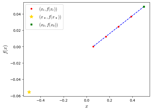
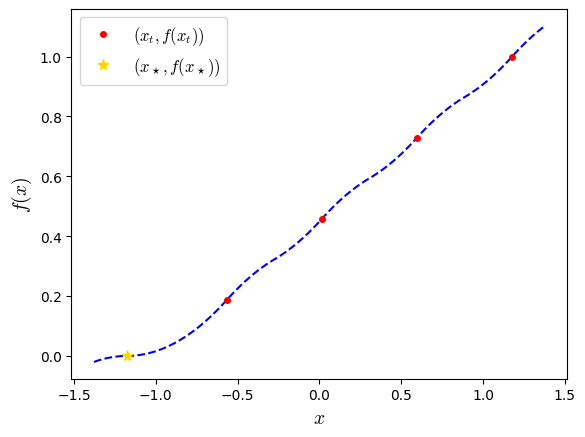
The last plot is giving a partial picture of what a worst-case function might look like: the function is evaluated only at a few points (iterates & an optimal point).
For this reason, we provide a few tools that allows extrapolating within certain classes of functions. This is done via the “interpolator” classes (that internally formulate the interpolation problems for a few classes).
The interpolator that corresponds to the PEP under consideration can be obtained (when implemented for the corresponding class) as follows (possibly with a few options):
feval = f.get_interpolator()
Now, we can evaluate an interpolating function on a grid of points “x_test” around the iterates and the solution.
# Create a grid of points where an interpolating function should be computed:
nb_pts_grid = 100
x_min = np.min([x0_evaluated,xs_evaluated])
x_max = np.max([x0_evaluated,xs_evaluated])
x_test = np.linspace(x_min,x_max,nb_pts_grid)

# Use the interpolation tools: evaluate a function using the "feval" interpolator on the grid:
fx_test = np.zeros(x_test.shape)
for i in range(len(x_test)):
    fx_test[i] = feval(np.array([x_test[i]]))
    print(f'{i + 1} / {len(x_test)} grid points computed', end='\r', flush=True)
100 / 100 grid points computed
… which we can now plot!
#plt.plot(x_list_evaluated[::1,], f_list_evaluated, '.--', color='blue')
plt.plot(x_test, fx_test, '--', color='blue', label='$(x,f(x))$')
plt.plot(x_list_evaluated, f_list_evaluated, marker='.', color='red',  linestyle='none', markersize=8, label='$(x_t,f(x_t))$')
plt.plot(xs_evaluated, fs_evaluated, marker='*', color='gold', linestyle='none', markersize=8, label=r'$(x_\star,f(x_\star))$')


plt.legend()
plt.xlabel('$x$')
plt.ylabel('$f(x)$')

plt.show()
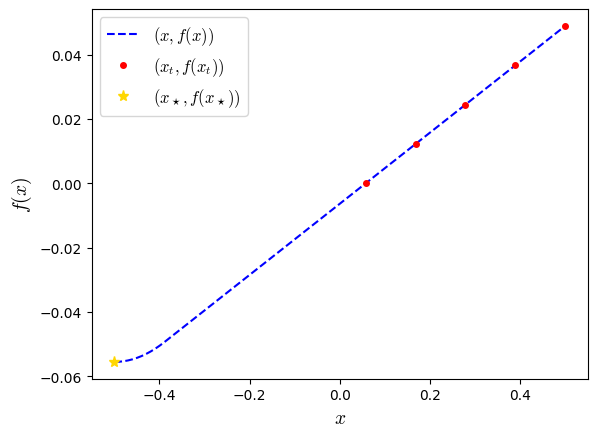
We observe a trajectory that looks like a type of Huber loss function, as predicted by the proof of Theorem 3.2 from this paper.
Example 2 : FISTA for composite convex minimization
We consider the following convex minimization problem:
where \(f\) is \(L\)-smooth and convex, and where \(h\) is convex (closed, proper) with a proximal operator readily available.
For this example, we consider the problem of computing the smallest possible \(\tau(n, L)\) such that the following guarantee holds (for any initialization of the algorithm, and any \(L\)-smooth convex function)
where \(x_n\) is the output of the FISTA initiated at \(x_0\), and where \(x_\star\) is a minimizer of \(F\).
Algorithm
The iterates of FISTA are described as (for \(t \in \{0,1, \ldots, n-1\}\))
Let us first start by importing all the necessary packages for the implementation in PEPit (this is done there, which we use below).
from math import sqrt
from PEPit import PEP
from PEPit.functions import SmoothConvexFunction
from PEPit.functions import ConvexFunction
from PEPit.primitive_steps import proximal_step
The following lines adapt the previous code to the study of FISTA:
# Parameters / options for the study:
verbose = 1  # verbose
n = 3 # number of iterations
L = 1 # Lipschitz constant

# Performance estimation problem (PEP) formulation:

# Instantiate PEP
problem = PEP()

# Declare a strongly convex smooth function and a convex function
f = problem.declare_function(SmoothConvexFunction, L=L)
h = problem.declare_function(ConvexFunction)
F = f + h

# Start by defining an optimal point xs = x_* and its function value Fs = F(x_*)
xs = F.stationary_point()
Fs = F(xs)
gs, fs = f.oracle(xs) # this is g(xs)=f'(x_*)
ss, hs = -gs, Fs - fs # this is s(xs) \in \partial h(x_*)  and hs = Fs - fs

# Create empty lists for saving a worst-case trajectory
y_list = list() # list of points where we will evaluate f() and its gradient
g_list = list() # list of evaluated gradients of f() at y's
f_list = list() # list of evaluated f() at y's
x_list = list() # list of outputs of the proximal operator
s_list = list() # list of evaluated subgradients of h() at x's (outputs of prox)
h_list = list() # list of evaluated h() at x's (outputs of prox)

# Then define a starting point x0
x0 = problem.set_initial_point()
g0, f0 = f.oracle(x0)
# Set the initial constraint that is the distance between x0 and x^*
problem.set_initial_condition((x0 - xs) ** 2 <= 1)

# Compute n steps of FISTA starting from x0
x_new = x0
y = x0
lam = 1
for i in range(n):
    # update momentum parameters
    lam_old = lam
    lam = (1 + sqrt(4 * lam_old ** 2 + 1)) / 2

    # save old point for momentum
    x_old = x_new

    # evaluate gradient at y + save corresponding values
    gy, fy = f.oracle(y)
    y_list.append(y)
    g_list.append(gy)
    f_list.append(fy)

    # perform a proximal-gradient step
    x_new, sx_new, hx_new = proximal_step(y - 1 / L * gy, h, 1 / L)

    # save outputs/subgradient of h() at x (output of prox)
    x_list.append(x_new)
    s_list.append(sx_new)
    h_list.append(hx_new)

    y = x_new + (lam_old - 1) / lam * (x_new - x_old)

# Since we evaluate the performance of the algorithm at x_n, we add it to the y_list (list of points at which f() is evaluated)
gx, fx = f.oracle(x_new)
y_list.append(x_new)
g_list.append(gx)
f_list.append(fx)

# Set the performance metric to the function value accuracy
problem.set_performance_metric((fx + hx_new) - Fs)

# Solve the PEP
pepit_verbose = max(verbose, 0)
pepit_tau = problem.solve(verbose=pepit_verbose, dimension_reduction_heuristic="trace", tol_dimension_reduction=1e-6)
(PEPit) Setting up the problem: performance measure is the minimum of 1 element(s)
(PEPit) Setting up the problem: Adding initial conditions and general constraints ...
(PEPit) Setting up the problem: initial conditions and general constraints (1 constraint(s) added)
(PEPit) Setting up the problem: interpolation conditions for 2 function(s)
			Function 1 : Adding 20 scalar constraint(s) ...
			Function 1 : 20 scalar constraint(s) added
			Function 2 : Adding 12 scalar constraint(s) ...
			Function 2 : 12 scalar constraint(s) added
(PEPit) Setting up the problem: additional constraints for 0 function(s)
(PEPit) Setting up the problem: size of the Gram matrix: 10x10
(PEPit) Compiling SDP
(PEPit) Calling SDP solver
(PEPit) Solver status: optimal (wrapper:cvxpy, solver: MOSEK); optimal value: 0.0761787865456547
(PEPit) Postprocessing: 3 eigenvalue(s) > 7.47573367793566e-08 before dimension reduction
(PEPit) Calling SDP solver
(PEPit) Solver status: optimal (solver: MOSEK); objective value: 0.07617778646356368
(PEPit) Postprocessing: 1 eigenvalue(s) > 3.6860755232230394e-09 after dimension reduction
(PEPit) Postprocessing: solver's output is not entirely feasible (smallest eigenvalue of the Gram matrix is: -9.4e-11 < 0).
 Small deviation from 0 may simply be due to numerical error. Big ones should be deeply investigated.
 In any case, from now the provided values of parameters are based on the projection of the Gram matrix onto the cone of symmetric semi-definite matrix.
(PEPit) Primal feasibility check:
		The solver found a Gram matrix that is positive semi-definite up to an error of 9.395236189612535e-11
		All the primal scalar constraints are verified up to an error of 1.9884285537563606e-10
(PEPit) Dual feasibility check:
		The solver found a residual matrix that is positive semi-definite
		All the dual scalar values associated with inequality constraints are nonnegative
(PEPit) The worst-case guarantee proof is perfectly reconstituted up to an error of 5.799556179640622e-08
(PEPit) Final upper bound (dual): 0.0761787908371793 and lower bound (primal example): 0.07617778646356368
(PEPit) Duality gap: absolute: 1.0043736156095662e-06 and relative: 1.3184599635091319e-05
Let us clean and evaluate the different lists, in order to plot the corresponding functions:
# Evaluation of the trajectories:
y_list_evaluated = [y.eval()[0] for y in y_list] # centered iterates (evaluations of f() )
x_list_evaluated = [x.eval()[0] for x in x_list] # centered iterates (evaluations of h() )

g_list_evaluated = [g.eval()[0] for g in g_list] # gradient values for f
s_list_evaluated = [s.eval()[0] for s in s_list] # gradient values for h

f_list_evaluated = [f.eval() for f in f_list] # centered function values
h_list_evaluated = [h.eval() for h in h_list] # centered function values

# Evaluations at the optimal point:
xs_evaluated = xs.eval()[0] # x*
gs_evaluated = gs.eval()[0] # g(x*)=0
fs_evaluated = fs.eval() # f(x*)
ss_evaluated = -gs_evaluated # s(x*) \in\partial h(x*)
hs_evaluated = Fs.eval()

# Evaluations at x0
x0_evaluated = x0.eval()[0] # x*
g0_evaluated = g0.eval()[0] # g(x*)=0
f0_evaluated = f0.eval() # f(x*)
Let us now plot the iterates on the two functions (in terms of \((y,f(y))\) and \((x,f(x))\), side to side:
import matplotlib.pyplot as plt

fig, (ax1, ax2) = plt.subplots(1, 2, figsize=(12, 5))

# --------------------------
# LEFT: trajectory evaluated on f()
# --------------------------
ax1.plot(y_list_evaluated, f_list_evaluated, '.--', color='blue')
ax1.plot(y_list_evaluated, f_list_evaluated, marker='.', color='red',
         linestyle='none', markersize=8,
         label='$\\{(y_t,f(y_t))\\}_{t=0,\\ldots,n} \\cup \\{(x_n,f(x_n))\\}$')
ax1.plot(xs_evaluated, fs_evaluated, marker='*', color='gold',
         linestyle='none', markersize=8,
         label='$(x_\\star,f(x_\\star))$')

ax1.set_xlabel('$x$')
ax1.set_ylabel('$f(x)$')
ax1.legend()
ax1.set_title('Trajectory on $f$')


# --------------------------
# RIGHT: trajectory evaluated on h()
# --------------------------
ax2.plot(x_list_evaluated, h_list_evaluated, '.--', color='blue')
ax2.plot(x_list_evaluated, h_list_evaluated, marker='.', color='red',
         linestyle='none', markersize=8,
         label='$\\{(x_t,h(x_t))\\}_{t=1,\\ldots,n}$')
ax2.plot(xs_evaluated, hs_evaluated, marker='*', color='gold',
         linestyle='none', markersize=8,
         label='$(x_\\star,h(x_\\star))$')

ax2.set_xlabel('$x$')
ax2.set_ylabel('$h(x)$')
ax2.legend()
ax2.set_title('Trajectory on $h$')

plt.tight_layout()
plt.show()
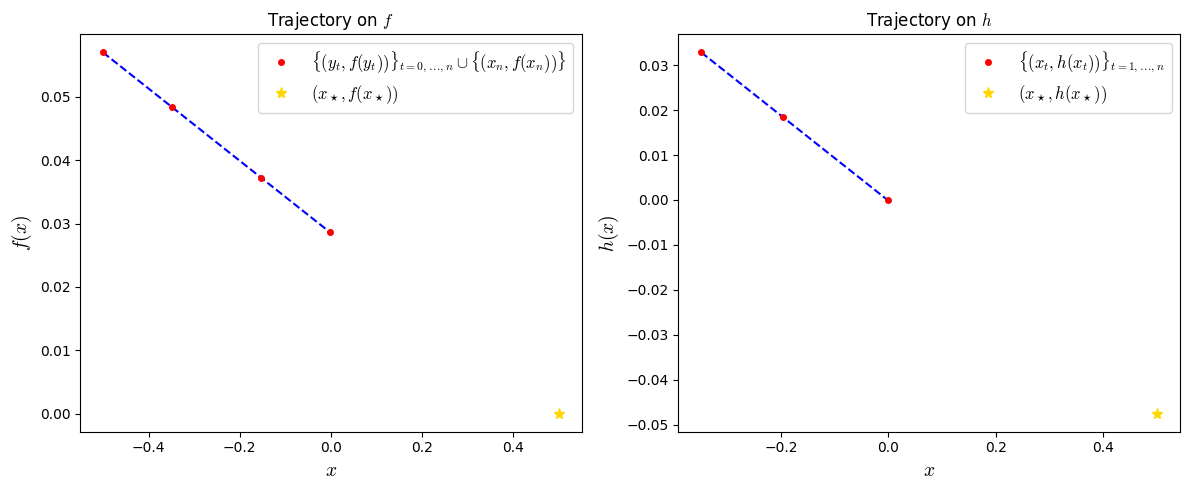
This is already quite informative, but arguably not enough. Can we easily recover a pair of functions interpolating through those points? Lets interpolate an example of a worst-case function \(F\) by computing the two functions \(f\) and \(g\) separately, again using the interpolator tool, which we instantiate below.
feval = f.get_interpolator()
heval = h.get_interpolator()
# Grid parameters
nb_pts_grid = 50
margin = .2 # plot the interpolated function slightly outside the convex hull of iterates/optimal point

# Create a grid of points where an interpolating function for f() should be computed:
y_min = np.min([np.min(y_list_evaluated),xs_evaluated])
y_max = np.max([np.max(y_list_evaluated),xs_evaluated])
y_test = np.linspace(y_min-margin,y_max+margin,nb_pts_grid)

fy_test = np.zeros(y_test.shape)
for i in range(len(y_test)):
    fy_test[i] = feval(np.array([y_test[i]]))
    print(f'{i + 1} / {len(y_test)} grid points computed', end='\r', flush=True)
50 / 50 grid points computed
# Create a grid of points where an interpolating function for h() should be computed:
nb_pts_grid = 50
x_min = np.min([np.min(x_list_evaluated),xs_evaluated])
x_max = np.max([np.max(x_list_evaluated),xs_evaluated])
x_test = np.linspace(x_min-margin,x_max+margin,nb_pts_grid)

hx_test = np.zeros(x_test.shape)
for i in range(len(x_test)):
    hx_test[i] = heval(np.array([x_test[i]]))
    print(f'{i + 1} / {len(x_test)} grid points computed', end='\r', flush=True)
50 / 50 grid points computed
The computed worst-case examples are thus as below:
import matplotlib.pyplot as plt

fig, (ax1, ax2) = plt.subplots(1, 2, figsize=(12, 5))

# --------------------------
# LEFT: trajectory evaluated on f()
# --------------------------
ax1.plot(y_test, fy_test, '--', color='blue')
ax1.plot(y_list_evaluated, f_list_evaluated, marker='.', color='red',
         linestyle='none', markersize=8,
         label='$\\{(y_t,f(y_t))\\}_{t=0,\\ldots,n} \\cup \\{(x_n,f(x_n))\\}$')
ax1.plot(xs_evaluated, fs_evaluated, marker='*', color='gold',
         linestyle='none', markersize=8,
         label='$(x_\\star,f(x_\\star))$')

ax1.set_xlabel('$x$')
ax1.set_ylabel('$f(x)$')
ax1.legend()
ax1.set_title('Trajectory on $f$')


# --------------------------
# RIGHT: trajectory evaluated on h()
# --------------------------
ax2.plot(x_test, hx_test, '--', color='blue')
ax2.plot(x_list_evaluated, h_list_evaluated, marker='.', color='red',
         linestyle='none', markersize=8,
         label='$\\{(x_t,h(x_t))\\}_{t=1,\\ldots,n}$')
ax2.plot(xs_evaluated, hs_evaluated, marker='*', color='gold',
         linestyle='none', markersize=8,
         label='$(x_\\star,h(x_\\star))$')

ax2.set_xlabel('$x$')
ax2.set_ylabel('$h(x)$')
ax2.legend()
ax2.set_title('Trajectory on $h$')

plt.tight_layout()
plt.show()
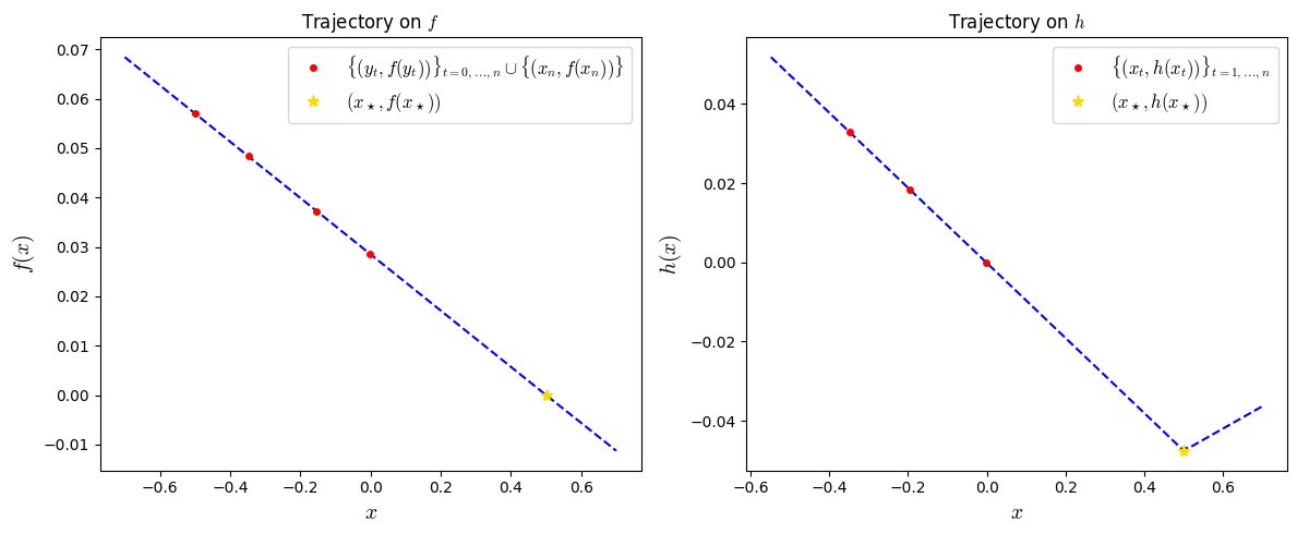
So we observe that the worst-case is achieved already when \(f\) is linear and when \(h\) is a \(\ell_1\)-shaped (in fact, a simple worst-case example of \(h\) is just the indicator function, see, e.g., this paper (Section 4.2) or Yoel Drori’s thesis, Section 2.8 for the related projected gradient method).
Example 3 : gradient descent for potentially non-convex minimization
We consider the following convex minimization problem:
where \(f\) is \(L\)-smooth (and potentially non-convex).
For this example, we consider the problem of computing the smallest possible \(\tau(n, L, \mu, \gamma)\) such that the following guarantee holds (for any initialization of the algorithm, and any \(L\)-smooth function)
where \(x_t\) are the iterates gradient descent with step size \(\gamma\), started from \(x_0\):
and where \(x_\star\) is a stationary point such that \(f(x_\star)\leq f(x_t)\) for all \(t=0,1,\ldots,n\).
from PEPit import PEP
from PEPit.functions import SmoothFunction

L = 1
n = 3
gamma = .95/L
verbose = 1


# Instantiate PEP
problem = PEP()

# Declare a smooth strongly convex function
f = problem.declare_function(SmoothFunction, L=L)

# Then define the starting point x0 of the algorithm as well as corresponding gradient and function value g0 and f0
x0 = problem.set_initial_point()
g0, f0 = f.oracle(x0)

xs = f.stationary_point()
gs, fs = f.oracle(xs)

# Run n steps of GD method with step-size gamma
x_list = list()
g_list = list()
f_list = list()
gx, fx = g0, f0

x_list.append(x0)
f_list.append(f0)
g_list.append(g0)

for i in range(n):
    # Set the performance metric to the minimum of the gradient norm over the iterations
    problem.set_performance_metric(gx**2)
    f.add_constraint(fs <= fx - 1/2/L * gx**2)
    x_list.append(x_list[-1] - gamma * gx)
    gx, fx = f.oracle(x_list[-1])
    f_list.append(fx)
    g_list.append(gx)
problem.set_performance_metric(gx**2)
f.add_constraint(fs <= fx - 1/2/L * gx**2)

# Set initial condition
problem.set_initial_condition( f0 - fs == 1)

# Solve the PEP
pepit_verbose = max(verbose, 0)
pepit_tau = problem.solve(verbose=pepit_verbose, dimension_reduction_heuristic="logdet3", tol_dimension_reduction=1e-6)
(PEPit) Setting up the problem: performance measure is the minimum of 4 element(s)
(PEPit) Setting up the problem: Adding initial conditions and general constraints ...
(PEPit) Setting up the problem: initial conditions and general constraints (1 constraint(s) added)
(PEPit) Setting up the problem: interpolation conditions for 1 function(s)
			Function 1 : Adding 20 scalar constraint(s) ...
			Function 1 : 20 scalar constraint(s) added
(PEPit) Setting up the problem: additional constraints for 1 function(s)
			Function 1 : Adding 4 scalar constraint(s) ...
			Function 1 : 4 scalar constraint(s) added
(PEPit) Setting up the problem: size of the Gram matrix: 6x6
(PEPit) Compiling SDP
(PEPit) Calling SDP solver
(PEPit) Solver status: optimal (wrapper:cvxpy, solver: MOSEK); optimal value: 0.37409398278086625
(PEPit) Postprocessing: 3 eigenvalue(s) > 2.4421028820441136e-07 before dimension reduction
(PEPit) Calling SDP solver
(PEPit) Solver status: optimal (solver: MOSEK); objective value: 0.3740929827808663
(PEPit) Postprocessing: 1 eigenvalue(s) > 1.69684698132068e-08 after 1 dimension reduction step(s)
(PEPit) Solver status: optimal (solver: MOSEK); objective value: 0.3740929827808663
(PEPit) Postprocessing: 1 eigenvalue(s) > 0 after 2 dimension reduction step(s)
(PEPit) Solver status: optimal (solver: MOSEK); objective value: 0.3740929827808663
(PEPit) Postprocessing: 1 eigenvalue(s) > 0 after 3 dimension reduction step(s)
(PEPit) Solver status: optimal (solver: MOSEK); objective value: 0.3740929827808663
(PEPit) Postprocessing: 1 eigenvalue(s) > 0 after dimension reduction
(PEPit) Postprocessing: solver's output is not entirely feasible (smallest eigenvalue of the Gram matrix is: -9.78e-11 < 0).
 Small deviation from 0 may simply be due to numerical error. Big ones should be deeply investigated.
 In any case, from now the provided values of parameters are based on the projection of the Gram matrix onto the cone of symmetric semi-definite matrix.
(PEPit) Primal feasibility check:
		The solver found a Gram matrix that is positive semi-definite up to an error of 9.78398866358543e-11
		All the primal scalar constraints are verified
(PEPit) Dual feasibility check:
		The solver found a residual matrix that is positive semi-definite
		All the dual scalar values associated with inequality constraints are nonnegative up to an error of 1.7054939895156864e-09
(PEPit) The worst-case guarantee proof is perfectly reconstituted up to an error of 1.0227133351078837e-08
(PEPit) Final upper bound (dual): 0.37409398344859657 and lower bound (primal example): 0.3740929827808663
(PEPit) Duality gap: absolute: 1.000667730288729e-06 and relative: 2.6749171365101323e-06
Again: PEPit claims to have found a 1D counterexample, so we focus on the first coordinates of the output.
# Evaluate the coordinate, gradient, and function values
x_list_evaluated = [x.eval()[0] for x in x_list]
g_list_evaluated = [g.eval()[0] for g in g_list]
f_list_evaluated = [f.eval() for f in f_list]

# Evaluate a specific point (x*):
xs_evaluated = xs.eval()[0] # x*
fs_evaluated = fs.eval() # f(x*)
gs_evaluated = gs.eval()[0] # g(x*)
Let us now obtain the interpolator and use it to visualize a worst-case instance!
# get an interpolator
feval = f.get_interpolator()


# Create a grid of points where an interpolating function for f() should be computed:
nb_pts_grid = 100 # number of points on the grid
margin = .2 # extrapolate outside only evaluated points

x_min = np.min([np.min(x_list_evaluated),xs_evaluated])
x_max = np.max([np.max(x_list_evaluated),xs_evaluated])
x_test = np.linspace(x_min-margin,x_max+margin,nb_pts_grid)

fx_test = np.zeros(x_test.shape)
# Interpolate on the grid!
for i in range(len(x_test)):
    fx_test[i] = feval(np.array([x_test[i]]))
    print(f'{i + 1} / {len(x_test)} grid points computed', end='\r', flush=True)
100 / 100 grid points computed
plt.plot(x_test, fx_test, '--', color='blue')
plt.plot(x_list_evaluated, f_list_evaluated, marker='.', color='red',  linestyle='none', markersize=8, label=r'$(x_t,f(x_t))$')
plt.plot(xs_evaluated, fs_evaluated, marker='*', color='gold', linestyle='none', markersize=8, label=r'$(x_\star,f(x_\star))$')


plt.legend()
plt.xlabel('$x$')
plt.ylabel('$f(x)$')

plt.show()
A natural question now is whether this interpolator is actually unique. In fact, it is not in general. In PEPit, the default interpolator is often the one that creates the lowest possible interpolating function (the one that results in points with the smallest possible function value), but one can configure the interpolator to do the opposite (as we shall see in the next example).
# get an interpolator
feval = f.get_interpolator(options='highest')


# Create a grid of points where an interpolating function for f() should be computed:
nb_pts_grid = 100 # number of points on the grid
margin = .2 # extrapolate outside only evaluated points

x_min = np.min([np.min(x_list_evaluated),xs_evaluated])
x_max = np.max([np.max(x_list_evaluated),xs_evaluated])
x_test = np.linspace(x_min-margin,x_max+margin,nb_pts_grid)

fx_test = np.zeros(x_test.shape)
# Interpolate on the grid!
for i in range(len(x_test)):
    fx_test[i] = feval(np.array([x_test[i]]))
    print(f'{i + 1} / {len(x_test)} grid points computed', end='\r', flush=True)
100 / 100 grid points computed
feval_lowest = f.get_interpolator()
fx_test_lowest = np.array([feval_lowest(np.array([x])) for x in x_test])

plt.plot(x_test, fx_test_lowest, '--', color='blue', label='Lowest interpolating function')
plt.plot(x_test, fx_test, '--', color='orange', label='Highest interpolating function')
plt.plot(x_list_evaluated, f_list_evaluated, marker='.', color='red',  linestyle='none', markersize=8, label='Shared interpolation points')
plt.plot(xs_evaluated, fs_evaluated, marker='*', color='gold', linestyle='none', markersize=8, label='Shared stationary point')


plt.legend()
plt.xlabel('$x$')
plt.ylabel('$f(x)$')

plt.show()
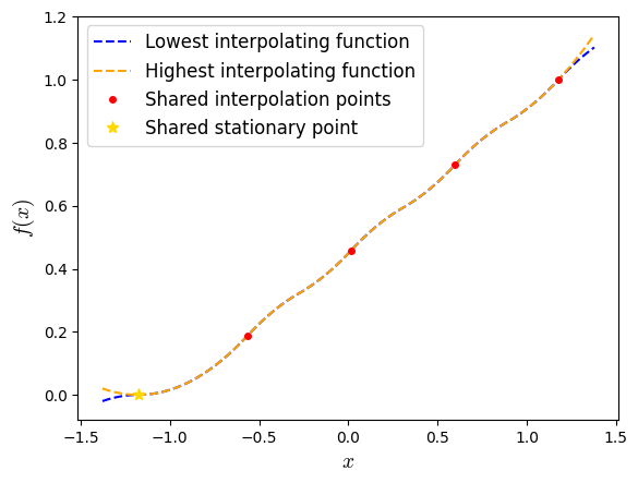
This is slightly different from the previous example (particularly outside of the range \([x_\star,x_0]\)).
Example 4 : alternate projections for finding a point in the intersection of two convex sets
In this example, we model the problem of finding a point in the intersection of two convex sets:
with \(f_1,f_2\) respectively the indicator functions for \(Q_1\) and \(Q_2\), which are closed convex sets.
More precisely, we investigate low-dimensional examples achieving a worst-case ratio for the criterion:
where \(x_t\) (\(t\in\{0,\ldots,n\}\)) are generated by the alternate projection method
We start by importing a few functions.
from PEPit import PEP
from PEPit.functions import ConvexIndicatorFunction
from PEPit.primitive_steps import proximal_step
# Parameters / options for the study:
verbose = 1  # verbose
n = 5 # number of iterations


# Instantiate PEP
problem = PEP()

f1 = problem.declare_function(ConvexIndicatorFunction) # indicator for Q1
f2 = problem.declare_function(ConvexIndicatorFunction) # indicator for Q2
func = f1 + f2 # indicator for the intersection

# x* is a point in the intersection
xs = func.stationary_point()

# Then define the starting point x0 of the algorithm
x0 = problem.set_initial_point()

# Run the alternate projection method
z_list = list() # list of points after projections
x = x0
for i in range(n):
    y, _, _ = proximal_step(x, f1, 1)
    z_list.append(y)
    x, _, _ = proximal_step(y, f2, 1)
    z_list.append(x)

# Set the performance metric to the distance between x and xs
problem.set_performance_metric((y-x)**2)
problem.set_initial_condition((x0-xs)**2==1)


# Solve the PEP
pepit_tau = problem.solve(verbose=verbose, dimension_reduction_heuristic='logdet2')
(PEPit) Setting up the problem: performance measure is the minimum of 1 element(s)
(PEPit) Setting up the problem: Adding initial conditions and general constraints ...
(PEPit) Setting up the problem: initial conditions and general constraints (1 constraint(s) added)
(PEPit) Setting up the problem: interpolation conditions for 2 function(s)
			Function 1 : Adding 36 scalar constraint(s) ...
			Function 1 : 36 scalar constraint(s) added
			Function 2 : Adding 36 scalar constraint(s) ...
			Function 2 : 36 scalar constraint(s) added
(PEPit) Setting up the problem: additional constraints for 0 function(s)
(PEPit) Setting up the problem: size of the Gram matrix: 13x13
(PEPit) Compiling SDP
(PEPit) Calling SDP solver
(PEPit) Solver status: optimal (wrapper:cvxpy, solver: MOSEK); optimal value: 0.04330493475326395
(PEPit) Postprocessing: 4 eigenvalue(s) > 1.3104667297245587e-07 before dimension reduction
(PEPit) Calling SDP solver
(PEPit) Solver status: optimal (solver: MOSEK); objective value: 0.043204935518465194
(PEPit) Postprocessing: 2 eigenvalue(s) > 5.7373804962052685e-09 after 1 dimension reduction step(s)
(PEPit) Solver status: optimal (solver: MOSEK); objective value: 0.04320493494675339
(PEPit) Postprocessing: 2 eigenvalue(s) > 0 after 2 dimension reduction step(s)
(PEPit) Solver status: optimal (solver: MOSEK); objective value: 0.04320493494675339
(PEPit) Postprocessing: 2 eigenvalue(s) > 0 after dimension reduction
(PEPit) Postprocessing: solver's output is not entirely feasible (smallest eigenvalue of the Gram matrix is: -5.09e-11 < 0).
 Small deviation from 0 may simply be due to numerical error. Big ones should be deeply investigated.
 In any case, from now the provided values of parameters are based on the projection of the Gram matrix onto the cone of symmetric semi-definite matrix.
(PEPit) Primal feasibility check:
		The solver found a Gram matrix that is positive semi-definite up to an error of 5.0896326265142404e-11
		All the primal scalar constraints are verified up to an error of 4.910116757628202e-11
(PEPit) Dual feasibility check:
		The solver found a residual matrix that is positive semi-definite
		All the dual scalar values associated with inequality constraints are nonnegative
(PEPit) The worst-case guarantee proof is perfectly reconstituted up to an error of 6.498126528869207e-08
(PEPit) Final upper bound (dual): 0.04330493817018899 and lower bound (primal example): 0.04320493494675339
(PEPit) Duality gap: absolute: 0.0001000032234355977 and relative: 0.0023146250204714724
As PEPit claims to have found a 2D example, we only visualize the first 2 coordinates of the identified worst-case instance.
# Evaluation at the optimal point:
xs_evaluated = xs.eval()[0:2] # x*

# Evaluation of the trajectories (centered around x* = 0 for simplicity)
z_list_evaluated = [z.eval()[0:2]-xs_evaluated[0:2] for z in z_list] # centered iterates

xs_evaluated = xs_evaluated - xs_evaluated # should be zero
z = np.array(z_list_evaluated)
x_points = np.vstack([x0.eval()[0:2] - xs.eval()[0:2], z[1::2]])
y_points = z[::2]
x_star = np.zeros(2)

# The worst-case sets are lines: find out their angle from the solution
q1_dir = y_points[np.argmax(np.sum(y_points**2, axis=1))]
q1_dir = q1_dir / np.linalg.norm(q1_dir)
q2_dir = x_points[1:][np.argmax(np.sum(x_points[1:]**2, axis=1))]
q2_dir = q2_dir / np.linalg.norm(q2_dir)

extent = 1.15 * np.max(np.abs(np.vstack([x_points, y_points, x_star])))
t = np.linspace(-extent, extent, 200)

fig, ax = plt.subplots(figsize=(8, 6))
ax.plot(t * q1_dir[0], t * q1_dir[1], '-.', color='tab:orange', lw=2, label=r'$Q_1$')
ax.plot(t * q2_dir[0], t * q2_dir[1], '--', color='tab:blue', lw=2, label=r'$Q_2$')

steps = [step for k in range(len(y_points))
         for step in ((x_points[k], y_points[k], 'tab:orange'),
                      (y_points[k], x_points[k + 1], 'tab:blue'))]
for i, (start, end, color) in enumerate(steps):
    if not np.allclose(start, end):
        ax.annotate('', xy=end, xytext=start,
                    arrowprops=dict(arrowstyle='-|>', color=color, lw=1.8, mutation_scale=12,
                                    shrinkA=0, shrinkB=4),
                    zorder=len(steps) - i)

y_plot = y_points[1:] if np.allclose(y_points[0], x_points[0]) else y_points
ax.scatter(x_points[1:, 0], x_points[1:, 1], color='tab:blue', s=60, edgecolors='black', linewidths=0.8, label=r'$x_t$', zorder=20)
ax.scatter(y_plot[:, 0], y_plot[:, 1], color='tab:orange', s=60, edgecolors='black', linewidths=0.8, label=r'$y_t$', zorder=20)
ax.scatter(*x_points[0], marker='s', color='green', s=120, edgecolors='black', linewidths=1.0, label=r'$x_0$', zorder=21)
ax.scatter(*x_star, marker='*', color='gold', s=220, edgecolors='goldenrod', linewidths=1.0, label=r'$x_\star$', zorder=21)

ax.set_xlabel('$z_1$')
ax.set_ylabel('$z_2$')
ax.set_aspect('equal', adjustable='box')
ax.legend()

plt.show()
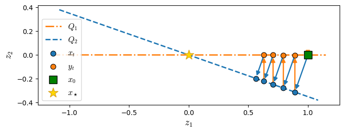
We observe a nice alternate projection between two hyperplanes! (and tuning the angle between the hyperplanes suffices to obtain the worst-case estimate)
Example 5 : primal-dual proximal point for convex minimization
For this last example, we consider again the problem of minimizing a sum:
where both \(f\) and \(h\) are closed convex and proper, and we assume \(\exists x_\star,y_\star\) (KKT point): \(-y_\star\in\partial f(x_\star),\, x_\star\in\partial h^*(y_\star)\).
We study the primal-dual (PD) proximal-point algorithm for solving such problems:
and we inspect guarantees of the form (for some elements of \(\partial f\) and \(\partial h^*\))
with \(g_N\in\partial f(x_N)\) and \(s_N\in\partial h^*(y_N)\).
To study this algorithm, we first import some necessary functions, followed by an implementation of the primal-dual proximal step in PEPit:
from PEPit import PEP
from PEPit.point import Point
from PEPit.expression import Expression
from PEPit.functions import ConvexFunction
import numpy as np

def PD_proximal_step(x0,lambda0, f, g, alpha):
    x1 = Point()
    lambda1 = Point()

    # subgradients
    pf_x1 = (x0-x1)/alpha-lambda1
    pg_lambda1 = (lambda0-lambda1)/alpha+x1

    fx1 = Expression()
    glambda1 = Expression()

    f.add_point((x1, pf_x1, fx1))
    g.add_point((pg_lambda1, lambda1, glambda1))

    return x1, lambda1, pf_x1, pg_lambda1

# helper function: evaluation of conjugate
def evaluate_conjugate(lam,f):
    x = Point()
    fx = Expression()
    f.add_point((x, lam, fx))
    fconj = lam*x - fx
    return fconj
n = 20 # number of iterations
alpha = n * [1] # step sizes
verbose = 1 # verbose mode


# PEP:
problem = PEP()

# Problem setup
f = problem.declare_function(ConvexFunction, reuse_gradient=True)
g = problem.declare_function(ConvexFunction, reuse_gradient=True)
F = f+g

# Optimal primal and dual solutions
xs = F.stationary_point()
ys = -f.gradient(xs)

# Starting point of the algorithm
x0 = problem.set_initial_point()
y0 = problem.set_initial_point()


# Compute n steps of the proximal method starting from x0
x_list = list()
y_list = list()
x_list.append(x0)
y_list.append(y0)

x = x0
y = y0
for i in range(n):
    x, y, df_xk, dg_lambdak = PD_proximal_step(x, y, f, g, alpha[i])
    x_list.append(x)
    y_list.append(y)

# Set initial condition (distance to a solution)
problem.set_initial_condition((x0 - xs) ** 2 + (y0 - ys) ** 2 <= 1)

# Set performance metric: KKT residual
problem.set_performance_metric((df_xk+y) ** 2 + (x - dg_lambdak) ** 2)

# Solve the PEP
pepit_tau = problem.solve(verbose=verbose, dimension_reduction_heuristic="logdet2")
(PEPit) Setting up the problem: performance measure is the minimum of 1 element(s)
(PEPit) Setting up the problem: Adding initial conditions and general constraints ...
(PEPit) Setting up the problem: initial conditions and general constraints (1 constraint(s) added)
(PEPit) Setting up the problem: interpolation conditions for 2 function(s)
			Function 1 : Adding 420 scalar constraint(s) ...
			Function 1 : 420 scalar constraint(s) added
			Function 2 : Adding 420 scalar constraint(s) ...
			Function 2 : 420 scalar constraint(s) added
(PEPit) Setting up the problem: additional constraints for 0 function(s)
(PEPit) Setting up the problem: size of the Gram matrix: 44x44
(PEPit) Compiling SDP
(PEPit) Calling SDP solver
(PEPit) Solver status: optimal (wrapper:cvxpy, solver: MOSEK); optimal value: 0.018867672516958034
(PEPit) Postprocessing: 6 eigenvalue(s) > 9.271131793728988e-08 before dimension reduction
(PEPit) Calling SDP solver
(PEPit) Solver status: optimal (solver: MOSEK); objective value: 0.01876767204806424
(PEPit) Postprocessing: 3 eigenvalue(s) > 0.005870284881130875 after 1 dimension reduction step(s)
(PEPit) Solver status: optimal (solver: MOSEK); objective value: 0.018767672468967378
(PEPit) Postprocessing: 2 eigenvalue(s) > 2.076211886853175e-11 after 2 dimension reduction step(s)
(PEPit) Solver status: optimal (solver: MOSEK); objective value: 0.018767672468967378
(PEPit) Postprocessing: 2 eigenvalue(s) > 2.076211886853175e-11 after dimension reduction
(PEPit) Postprocessing: solver's output is not entirely feasible (smallest eigenvalue of the Gram matrix is: -8.13e-11 < 0).
 Small deviation from 0 may simply be due to numerical error. Big ones should be deeply investigated.
 In any case, from now the provided values of parameters are based on the projection of the Gram matrix onto the cone of symmetric semi-definite matrix.
(PEPit) Primal feasibility check:
		The solver found a Gram matrix that is positive semi-definite up to an error of 8.129860241260612e-11
		All the primal scalar constraints are verified up to an error of 1.729408734274518e-10
(PEPit) Dual feasibility check:
		The solver found a residual matrix that is positive semi-definite
		All the dual scalar values associated with inequality constraints are nonnegative
(PEPit) The worst-case guarantee proof is perfectly reconstituted up to an error of 3.191634905460896e-08
(PEPit) Final upper bound (dual): 0.018867673113931446 and lower bound (primal example): 0.018767672468967378
(PEPit) Duality gap: absolute: 0.00010000064496406766 and relative: 0.005328345596899146
PEPit claims to have found a 2D counter-example, so let us only visualize the first two coordinates.
# Evaluate specific point (a solution)
xs_evaluated = xs.eval()[0:2] # x*
ys_evaluated = ys.eval()[0:2] # y*

# Evaluate the list of iterates (centered around the solution above, for simplificty)
x_list_evaluated = [x.eval()[0:2]-xs_evaluated for x in x_list] # centered iterates
xs_evaluated = xs_evaluated - xs_evaluated # should be zero
y_list_evaluated = [y.eval()[0:2]-ys_evaluated for y in y_list] # centered iterates
ys_evaluated = ys_evaluated - ys_evaluated # should be zero
Now, let us plot a worst-case trajectory!
import matplotlib
import matplotlib.pyplot as plt
%matplotlib widget
plt.ion()  # <-- this enables rotation


import numpy as np

# Convert the list of 2D vectors into two arrays x1, x2
x_array = np.array(x_list_evaluated)
x1 = x_array[:, 0]
x2 = x_array[:, 1]
# Convert the list of 2D vectors into two arrays y1, y2
y_array = np.array(y_list_evaluated)
y1 = y_array[:, 0]
y2 = y_array[:, 1]

# Worst-case point (xs_evaluated is a 2D vector)
xs = np.array(xs_evaluated)
xs1, xs2 = xs[0], xs[1]
# Worst-case point (ys_evaluated is a 2D vector)
ys = np.array(ys_evaluated)
ys1, ys2 = ys[0], ys[1]

fig = plt.figure(figsize=(9, 6))
ax = fig.add_subplot(111, projection='3d')

# Blue line (trajectory)
ax.plot(x1, y1, y2, '--', color='blue')
ax.scatter(x1, y1, y2, marker='o', color='red',
           s=20, label='$(x_t,y_t^{(1)},y_t^{(2)})$')

# Gold star (optimal point)
ax.scatter(xs1, ys1, ys2, marker='*', color='gold',
           s=100, label=r'$(x_\star,y_\star^{(1)},y_\star^{(2)})$')

# Green point (starting point)
ax.scatter(x1[0], y1[0], y2[0], marker='s', color='green',
           s=100, label='$(x_0,y_0^{(1)},y_0^{(2)})$')

ax.set_xlabel('$x^{(1)}$')
ax.set_ylabel('$y^{(1)}$')
ax.set_zlabel('$y^{(2)}$')

ax.legend(loc='upper center', bbox_to_anchor=(0.5, -0.08), ncol=3, borderaxespad=0.)
fig.subplots_adjust(bottom=0.2)

plt.show()
Example 6 : gradient descent with exact line-search
We now consider the problem of finding:
where \(f\) is \(L\)-smooth and \(\mu\)-strongly convex.
For this example, we consider the problem of computing the smallest possible \(\tau(n, L, \gamma)\) such that the following guarantee holds (for any initialization of the algorithm, and any \(L\)-smooth and \(\mu\)-strognly convex functions)
where \(x_n\) is the output of gradient descent using the per-iteration optimal step size \(\gamma_k = \arg\min_\gamma f(x_k) - \gamma \cdot \nabla f(x_k)\), started from \(x_0\), and where \(x_\star\) is the minimizer of \(f\).
from PEPit import PEP
from PEPit.functions import SmoothStronglyConvexFunction
from PEPit.primitive_steps import exact_linesearch_step

L, mu = 1, .1
verbose = 1
n = 5

# Instantiate PEP
problem = PEP()

# Declare a smooth strongly convex function
f = problem.declare_function(SmoothStronglyConvexFunction, mu=mu, L=L)

# Start by defining its unique optimal point xs = x_* and corresponding function value fs = f_*
xs = f.stationary_point()
gs, fs = f.oracle(xs)

# Then define the starting point x0 of the algorithm as well as corresponding gradient and function value g0 and f0
x0 = problem.set_initial_point()
g0, f0 = f.oracle(x0)

# Set the initial constraint that is the difference between f0 and f_*
problem.set_initial_condition(f0 - fs <= 1)

# Run n steps of GD method with ELS
x_list = list()
x_list.append(x0)
g_list = list()
g_list.append(g0)
f_list = list()
f_list.append(f0)

x = x0
gx = g0
for i in range(n):
    x, gx, fx = exact_linesearch_step(x, f, [gx])
    x_list.append(x)
    g_list.append(gx)
    f_list.append(fx)

# Set the performance metric to the function value accuracy
problem.set_performance_metric(fx - fs)

# Solve the PEP
pepit_verbose = max(verbose, 0)
pepit_tau = problem.solve(verbose=pepit_verbose, dimension_reduction_heuristic='trace')

# Compute theoretical guarantee (for comparison)
theoretical_tau = ((L - mu) / (L + mu)) ** (2 * n)
(PEPit) Setting up the problem: performance measure is the minimum of 1 element(s)
(PEPit) Setting up the problem: Adding initial conditions and general constraints ...
(PEPit) Setting up the problem: initial conditions and general constraints (1 constraint(s) added)
(PEPit) Setting up the problem: interpolation conditions for 1 function(s)
			Function 1 : Adding 42 scalar constraint(s) ...
			Function 1 : 42 scalar constraint(s) added
(PEPit) Setting up the problem: additional constraints for 1 function(s)
			Function 1 : Adding 10 scalar constraint(s) ...
			Function 1 : 10 scalar constraint(s) added
(PEPit) Setting up the problem: size of the Gram matrix: 13x13
(PEPit) Compiling SDP
(PEPit) Calling SDP solver
(PEPit) Solver status: optimal (wrapper:cvxpy, solver: MOSEK); optimal value: 0.1344305389387117
(PEPit) Postprocessing: 3 eigenvalue(s) > 5.4073880114545966e-06 before dimension reduction
(PEPit) Calling SDP solver
(PEPit) Solver status: optimal (solver: MOSEK); objective value: 0.13433053869743988
(PEPit) Postprocessing: 2 eigenvalue(s) > 6.004102165538769e-08 after dimension reduction
(PEPit) Postprocessing: solver's output is not entirely feasible (smallest eigenvalue of the Gram matrix is: -2.31e-10 < 0).
 Small deviation from 0 may simply be due to numerical error. Big ones should be deeply investigated.
 In any case, from now the provided values of parameters are based on the projection of the Gram matrix onto the cone of symmetric semi-definite matrix.
(PEPit) Primal feasibility check:
		The solver found a Gram matrix that is positive semi-definite up to an error of 2.3052389346073744e-10
		All the primal scalar constraints are verified up to an error of 3.7212867856628584e-10
(PEPit) Dual feasibility check:
		The solver found a residual matrix that is positive semi-definite
		All the dual scalar values associated with inequality constraints are nonnegative
(PEPit) The worst-case guarantee proof is perfectly reconstituted up to an error of 1.411303044625698e-07
(PEPit) Final upper bound (dual): 0.13443054662214557 and lower bound (primal example): 0.13433053869743988
(PEPit) Duality gap: absolute: 0.0001000079247056862 and relative: 0.0007444913545008525
As before, PEPit claims to have identified a 2D example. So we will focus on the first coordinates of the output vectors.
xs_evaluated = xs.eval()[0:2] # x*
gs_evaluated = gs.eval()[0:2] # g(x*)=0
fs_evaluated = fs.eval() # f(x*)

x_list_evaluated = [x.eval()[0:2] for x in x_list] # iterates
g_list_evaluated = [g.eval()[0:2] for g in g_list] # gradient values
f_list_evaluated = [f.eval() for f in f_list] # function values

x_list_evaluated.append(xs_evaluated)
g_list_evaluated.append(gs_evaluated)
f_list_evaluated.append(fs_evaluated)
We get the interpolator and interpolate on a grid:
feval = f.get_interpolator()

# Create a grid of points where an interpolating function for f() should be computed:
nb_pts_grid = 20 # number of points on the grid
margin = .2 # extrapolate outside only evaluated points

# x_list_evaluated is a list of numpy arrays
first_coordinate = np.array([arr[0] for arr in x_list_evaluated])
second_coordinate = np.array([arr[1] for arr in x_list_evaluated])

x_min, x_max = np.min(first_coordinate)-margin, np.max(first_coordinate)+margin
y_min, y_max = np.min(second_coordinate)-margin, np.max(second_coordinate)+margin

# Create test points
x_test = np.linspace(x_min, x_max, nb_pts_grid)
y_test = np.linspace(y_min, y_max, nb_pts_grid)

# Create 2D mesh
X, Y = np.meshgrid(x_test, y_test)

# Array to store function evaluations
FX = np.zeros(X.shape)

# Loop over the mesh
for i in range(X.shape[0]):
    for j in range(X.shape[1]):
        x_tested = np.zeros((7,))
        x_tested[0] = X[i, j]
        x_tested[1] = Y[i, j]
        FX[i, j] = feval(x_tested)

        print(f'{i * X.shape[1] + j + 1} / {X.size} mesh points computed', end='\r', flush=True)
400 / 400 mesh points computed
Now, let us plot the function; first with a contour plot (a bit more readable), then followed by a surface plot.
import matplotlib.pyplot as plt
import numpy as np

# Create figure and axes (2D now)
fig, ax = plt.subplots(figsize=(8,6))

# Contour plot
cont = ax.contourf(X, Y, FX, levels=50, cmap='viridis')

# Extract x, y from x_list_evaluated
x_pts = np.array([arr[0] for arr in x_list_evaluated])
y_pts = np.array([arr[1] for arr in x_list_evaluated])

# Overlay evaluated points (more visible)
ax.plot(
    x_pts[:-1],
    y_pts[:-1],
    color='green',
    linewidth=2.5,
    label='Trajectory'
)
ax.scatter(
    x_pts[:-1],
    y_pts[:-1],
    color='red',
    s=150,
    edgecolors='black',
    linewidths=1.5,
    marker='o',
    label='Iterates'
)
ax.scatter(
    x_pts[0],
    y_pts[0],
    color='green',
    s=150,
    edgecolors='black',
    linewidths=1.5,
    marker='s',
    label='Starting point'
)
ax.scatter(
    x_pts[-1],
    y_pts[-1],
    color='gold',
    s=150,
    edgecolors='black',
    linewidths=1.5,
    marker='*',
    label='Optimal point'
)

# Color bar
cbar = fig.colorbar(cont, ax=ax, orientation='horizontal', location='top', pad=0.08, label='f(x)')

# Labels
ax.set_xlabel(r'$x^{(1)}$')
ax.set_ylabel(r'$x^{(2)}$')

# Title
ax.set_title('Contour plot of f(x)')

ax.legend()

plt.show()
import matplotlib.pyplot as plt
from mpl_toolkits.mplot3d import Axes3D
import numpy as np

# Create figure and 3D axes
fig = plt.figure(figsize=(9,6))
ax = fig.add_subplot(111, projection='3d', computed_zorder=False)

# Plot the surface
surf = ax.plot_surface(
    X, Y, FX,
    cmap='viridis',
    edgecolor='none',
    alpha=0.8,
    zorder=0
)

# Extract x, y from x_list_evaluated
x_pts = np.array([arr[0] for arr in x_list_evaluated])
y_pts = np.array([arr[1] for arr in x_list_evaluated])
z_pts = np.array(f_list_evaluated)

# Overlay evaluated points (more visible)
ax.plot(
    x_pts[:-1],
    y_pts[:-1],
    z_pts[:-1],
    color='green',
    linewidth=2.5,
    zorder=5,
    label='Trajectory'
)
ax.scatter(
    x_pts[:-1],
    y_pts[:-1],
    z_pts[:-1],
    color='red',
    s=150,
    edgecolors='black',
    linewidths=1.5,
    depthshade=False,
    marker='o',
    zorder=10,
    label='Iterates'
)
ax.scatter(
    x_pts[0],
    y_pts[0],
    z_pts[0],
    color='green',
    s=150,
    edgecolors='black',
    linewidths=1.5,
    depthshade=False,
    marker='s',
    zorder=10,
    label='Starting point'
)
ax.scatter(
    x_pts[-1],
    y_pts[-1],
    z_pts[-1],
    color='gold',
    s=150,
    edgecolors='black',
    linewidths=1.5,
    depthshade=False,
    marker='*',
    zorder=10,
    label='Optimal point'
)

# Add color bar
fig.colorbar(surf, ax=ax, orientation='horizontal', location='top', pad=0.02, shrink=0.42, aspect=30, label='$f(x)$')

# Labels
ax.set_xlabel(r'$x^{(1)}$')
ax.set_ylabel(r'$x^{(2)}$')
ax.set_zlabel('$f(x)$')

# Title
fig.suptitle('Surface plot of $f(x)$', y=0.93)

ax.legend(loc='upper center', bbox_to_anchor=(0.5, -0.08), ncol=2, borderaxespad=0.)
fig.subplots_adjust(bottom=0.2, top=0.87)

plt.show()